How to Use Data Validation Formula in Google Sheets?

The Data Validation formula in Google Sheets allows you to set criteria that are not included in any Data Validation criteria types.

If you’ve never used the Data Validation formula in Google Sheets, don’t worry; you have come to the right place.

Continue reading to learn how to use the Data Validation formula in Google Sheets.

How to Use Data Validation Formula in Google Sheets?

Data Validation custom formula in Google Sheets allows you to set certain parameters on your own to prevent making input errors.

There are different ways to use Data Validation on Google Sheets, such as from a list of items, numbers, Data, checkboxes, custom formulas, etc.

You can create a Data Validation formula on Google Sheets which allows you to enter your custom formula.

Follow these steps to use the function;

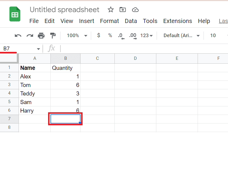
1. Open a Google spreadsheet.
2. Double-click the cells where you want to set up Data Validation.



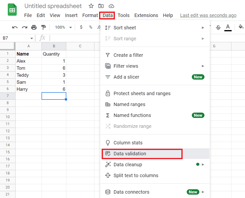
3. Go to Data > Data Validation.



4. Click Plus(+) button to add a Validation rule.



5. Click the drop-down icon of the Criteria option.
6. Select the range if necessary.
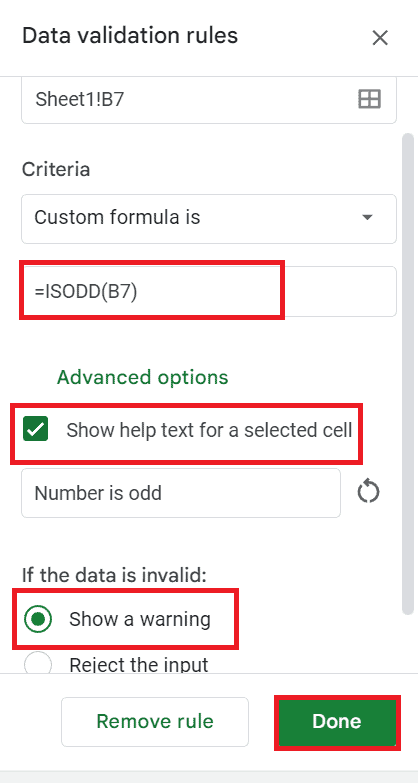
7. Select “Custom Formula is” and set up your formula.
8. For example, use “=ISODD(B7)” on the box. Here A1 is the representation of the cell.
9. You can choose Appearance. Tick Show Validation help text. Enter any text (For e.g., Number is odd)
10. Finally, click the Save button.



11. You can see a red symbol inside the cell with an error message if the entered value is even.



12. If the entered value is odd, then no error message is displayed.

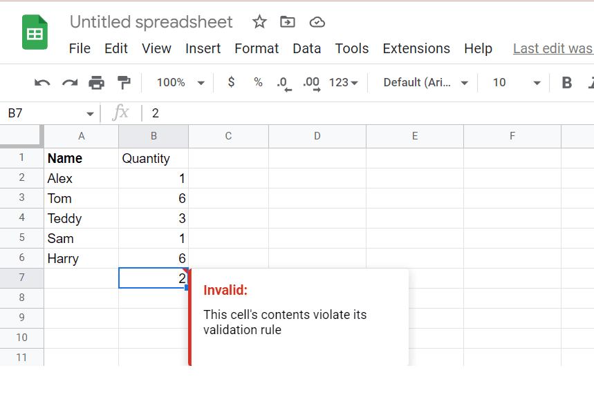
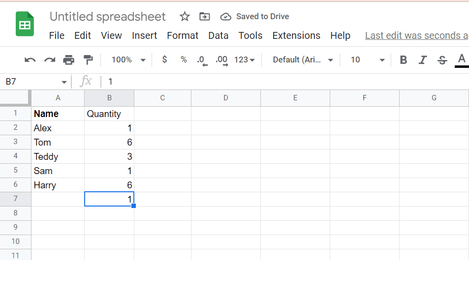
This is just an example of one formula for cell B7. The custom formula can be much more complex than the example shown above.

You can customize many formulas and use them in your Google Sheets.

Data Validation in Google Sheets Using Custom Formula

To understand the Data Validation custom formula, first, you need to understand cell references.

1. Relative Cell References

• All call references are relative by default.
• Relative cell references change when a formula is copied to another cell.
• It is appropriate whenever you need to repeat the same calculation.

2. Absolute Cell References

• Remain constant when a formula is copied to another cell. No matter from which cell they are copied, it remains constant.
• It is appropriate whenever you need to keep row/column constant.
• The dollar sign ($) plays a vital role in Absolute Cell References.
• The cell reference remains constant if you use the dollar sign when you copy.

Example of Custom Formulas in Google Sheet Data Validation

Let’s start with the basic example of how to use custom formulas in Data Validation in Google Sheets.

Here are some examples of custom formulas.

=isodd(A1)

This formula changes the function ISODD with ISEVEN and allows only even numbers.

=and(iseven(A1), B1=”Yes”)

This formula allows only even numbers in the range A1:An if the range B1:Bn contains “Yes.” (Here, n is a number of selected ranges)

=$A$1=”Allow”

This formula removes the word Allow from one cell (let A1 ) and then types on another cell in the Data Validation range.

An error will occur if you do not have the word ‘Allow’ in A1.

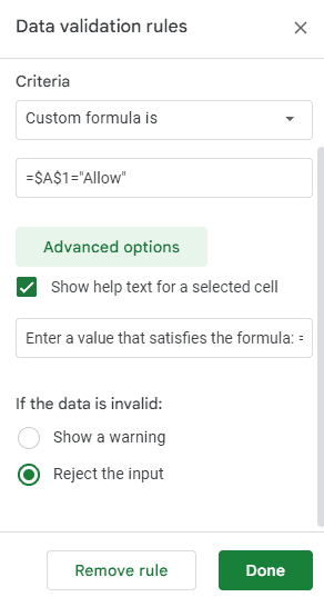
If you type the ‘Allow’ word in A1, you can enter Data into the Data Validation range of cells.

=$A$1=”No”

If the cell A1 equals “No,” then Data will be accepted for the range of Data Validation.

As mentioned above, $ represents an absolute cell reference to cell A1.

If A1 equals anything other than “No,” it will reject any input.

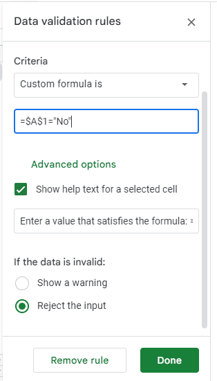
In case A1 is set to “Yes,” and you enter Data in the highlighted cells, you will see There was a problem message in your window.

Data Validation Custom Formula With VLOOKUP Function

VLOOKUP is simply a vertical lookup function.

The VLOOKUP function in Google Sheets allows you to search for an item across columns and return Data from the row using a specified search key.

The VLOOKUP function in Google Sheets works the same as in Excel.

Here are some rules for using the VLOOKUP function in Google Sheets;

• Search_key can be any of the cells in the column except the last one.
• The range is to search the index, which is the number of columns from the Data extracted.
• The index is 1 for the first column of the range, 2 for the second column of the range, and so on.
• Optional is sorted, and its value will be true if the column is sorted and false if it is not sorted in the closing brackets.

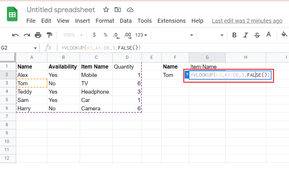
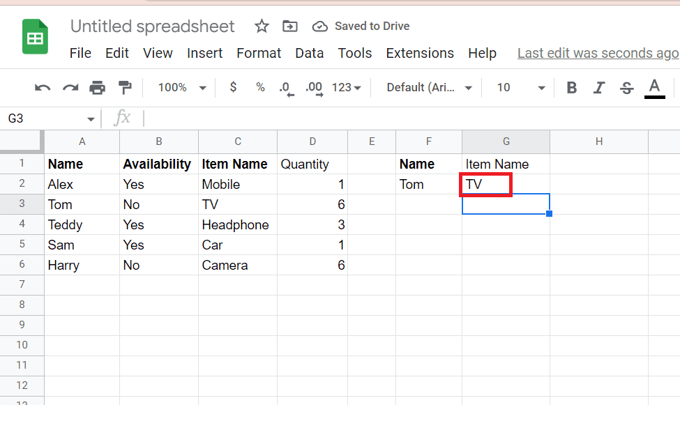
For example, we can use the VLOOKUP formula to search for TV in column 3.

When the result matches the search value, it will return the value from the sixth column to give the value 52.

1. Insert the VLOOKUP formula as per your requirements. Specify the search key, range, index, etc.
2. We use False() in the is_sorted option because we need an exact match.



3. After inserting the VLOOKUP formula in the cell, Press enter button.
4. You can see the item name as TV on the corresponding cell.

The Bottom Line

Custom formula Data Validation is one of the most important functions in Google Sheets for Data analysts and others.

I hope the above procedures will be sufficient to use Google Sheet Data Validation with a custom formula.